File Structure
Circuit of the RC filter.We simulated a simple RC filter in LTSPICE. With the simple RC Filter we tested each option in LTSPICE.There are 4 different options to simulate a circuit: ".tran" is the transient simulation. Here we have to set the stop time, the time step and time to saving data. ".ac" is the as analysis. Here we set the start, the stop frequency and the sweep type. ".op" is for the DC operation point of a circuit. LTSPICE supports three other simulation commands. But we just focused on this three types. For the hand calculation of the cut off frequency we use the following formula: fc = 1/(2*Pi*R*C) |
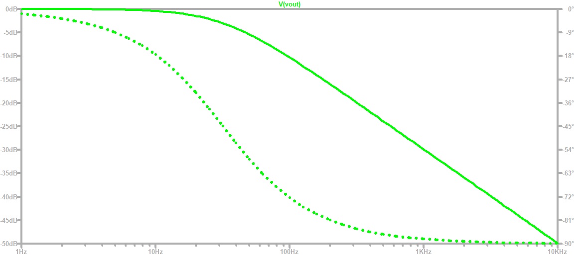
Transfer Curve of the RC FilterFrom the transfer curve we could extract the 3dB cut off frequency.The frequency we extracted from the curve was matching with our hand calculation. As we are simulating an ideal ADC and DAC there is no deviation between each step. |
|
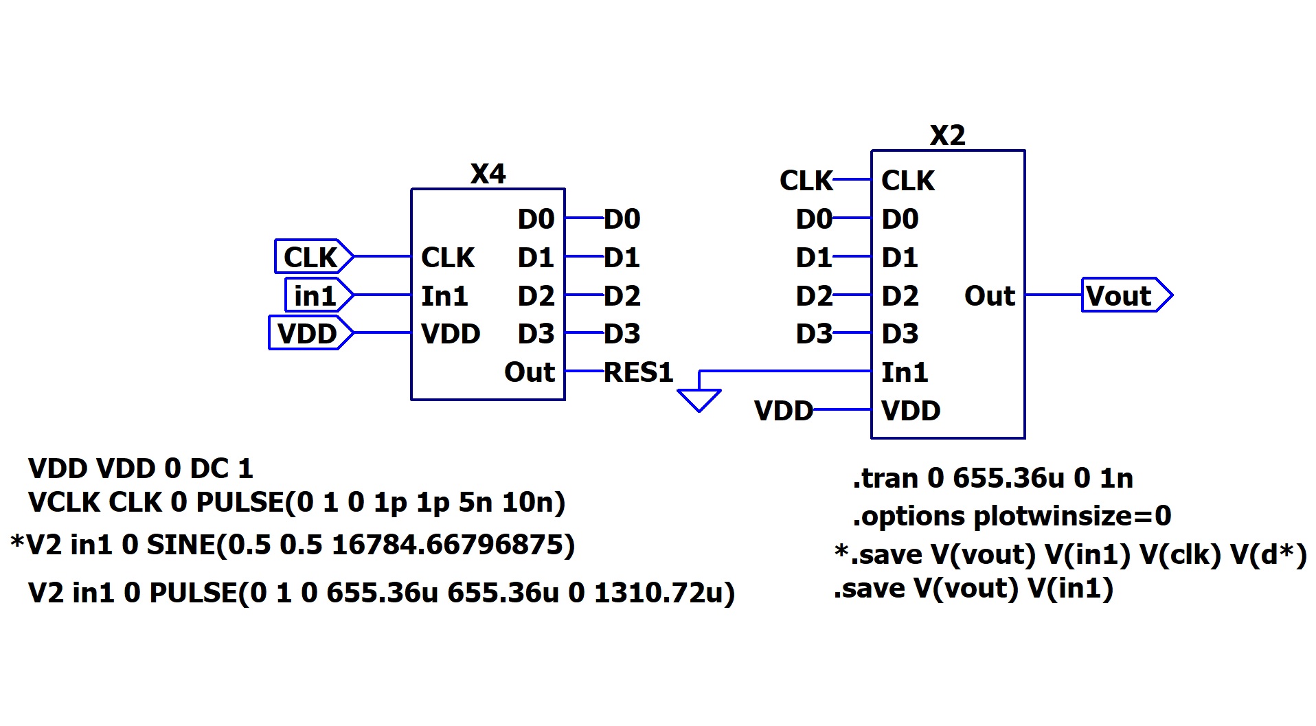
DP Chart of the ADC_DAC Pipe.We used this schematic for the simulation of an ADC_DAC pipe.The following slides are explaining all our simulations more in detail. Since the javascript tool has problems with loading LTSPICE Symbols in LTSPICE schematics here is only a screenshot used. |
|
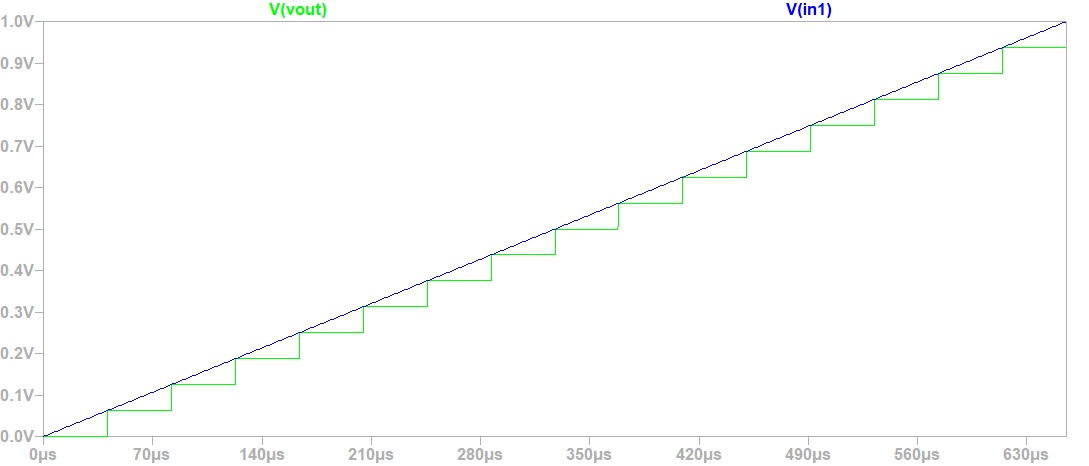
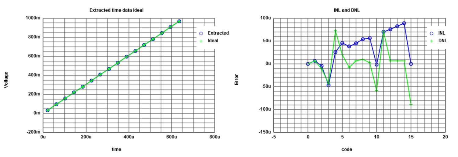
Ramp Simulation.The picture beside shows the result of out ramp simulation with the ADC_DAC_Pipe.With a ramp as input signal we are able to extract the switching voltage between each bit. As we are simulating an ideal ADC and DAC there is no deviation between each step. |
|
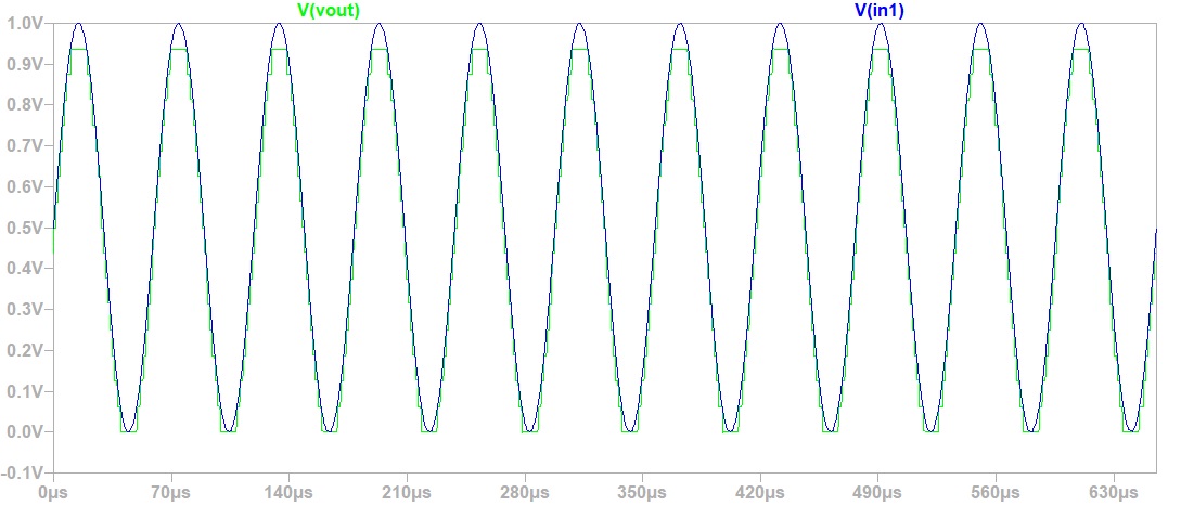
Sine Simulation.The picture beside shows our result of the sine simulation with the ADC_DAC_Pipe.The sine signal is much better to test an ADC or a DAC in real live, but it makes much more effort in analysing the result. |
|
INL DNL Chart of the ADC_DAC Pipe.INL and DNL simulation with Javascript tool from WebsiteFor this simulation a Ramp was used as input signal. Calculation of the DNL: DNL = (V(n) - V(n-1) - LSB) / LSB Calculation of the INL: INL = (Vreal(n) - Videal(n)) / LSB |
|
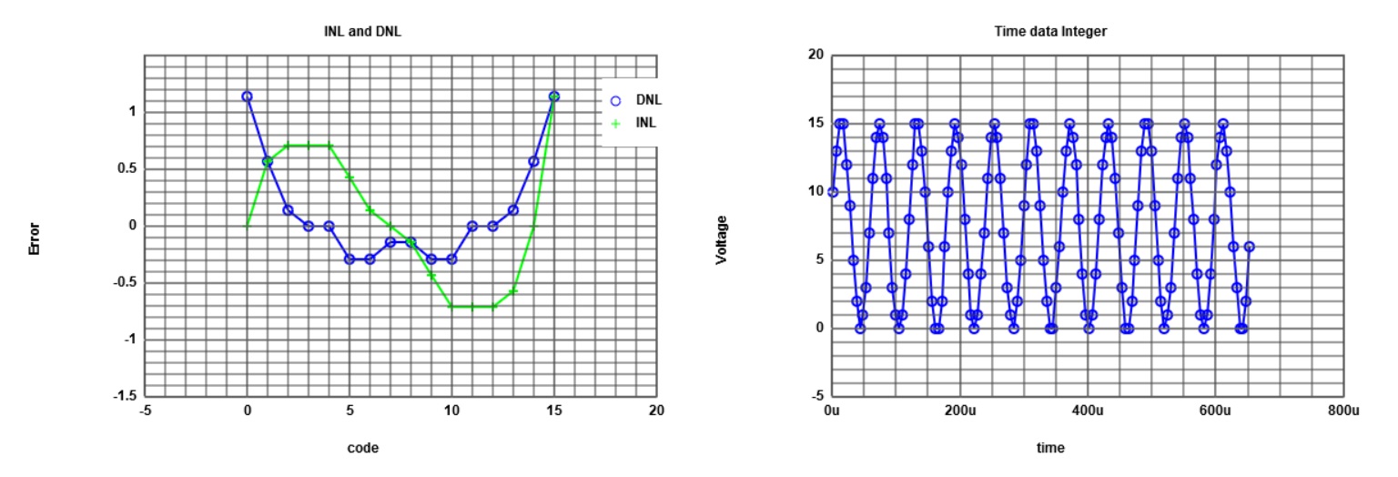
INL DNL Chart of the ADC_DAC Pipe.INL and DNL simulation with Javascript tool from WebsiteFor this simulation a Sine was used as input signal. Here the calculation of the DNL and the INL is done with the histogram calculation. With a sine signal a direct calculation is not possible. Out of the sine signal our result is not a linear curve. |
|
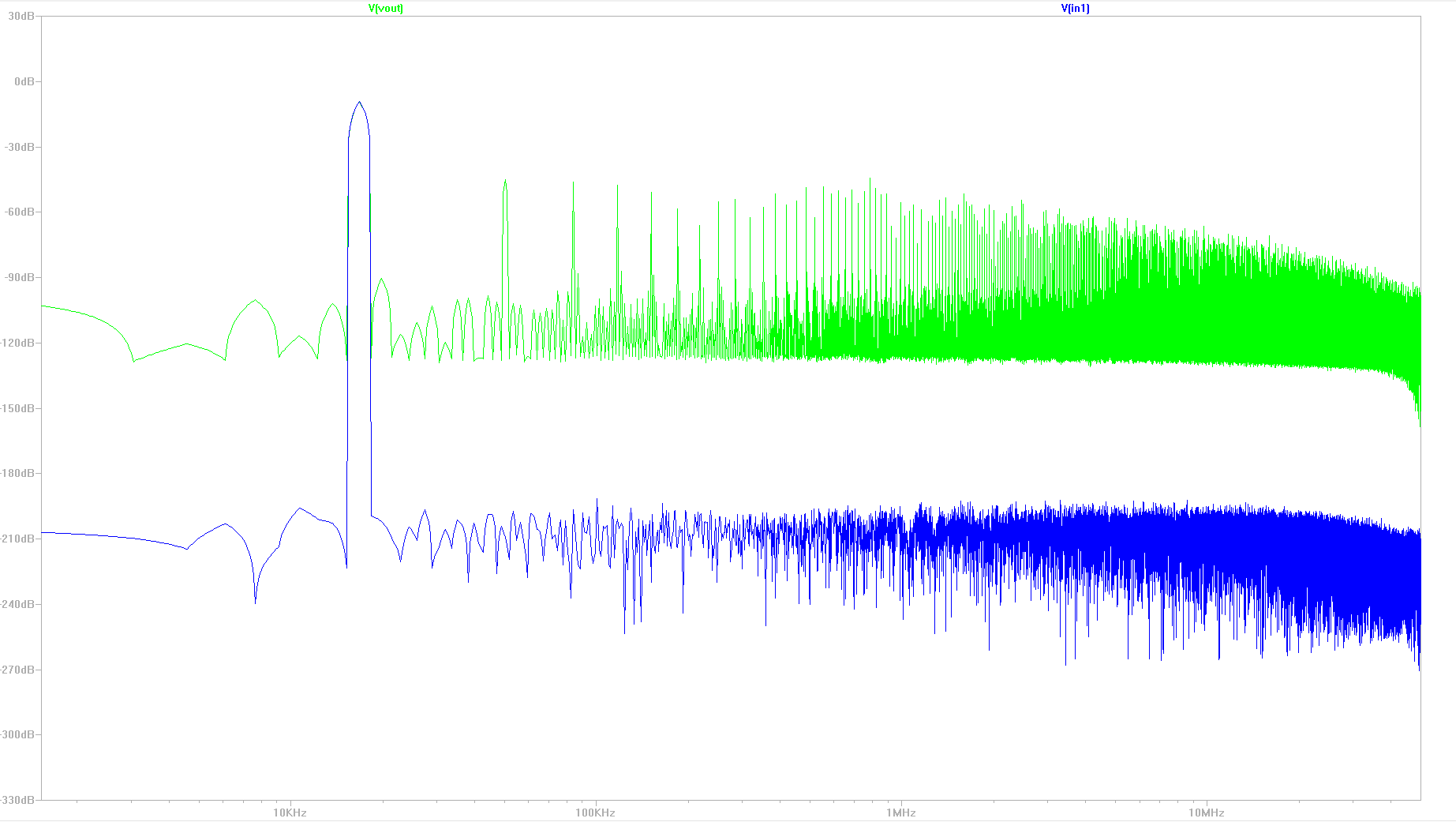
FFT of the ADC_DAC Pipe.The noise in the FFT is very high. This is due to the SNR of the only 4Bit ADC. This ADC/DAC kombination has only a very low Signal to Noise Ratio. If we would increase the number of Bits, the SNR would be much higher and we would be able to see clearly the frequency of the original Signal. In the image beside we could imagine the frequency of the original Signal. |
|
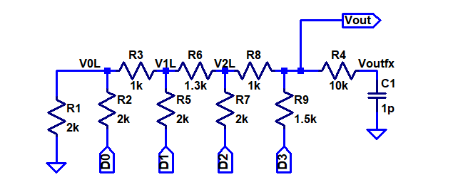
Circuit of the R2R Circuit.For the simulations of this circuit the ideal values of 2 resistors is changed.Therefore an error in the transfer curve occures. Thus, the difference between ideal and real transfer curve can be explained. |
|
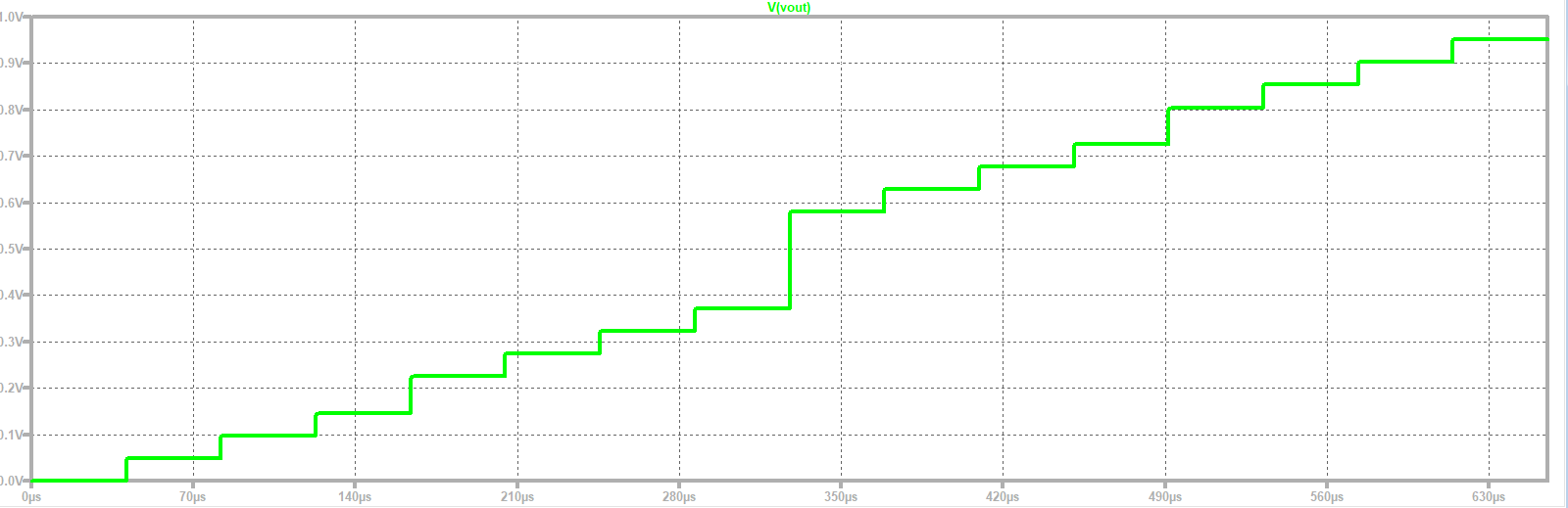
Transfer curves of the R2R DACRamp test simulation with LTSPICE.In this figure you can see the error due to the change in resistance. |
|
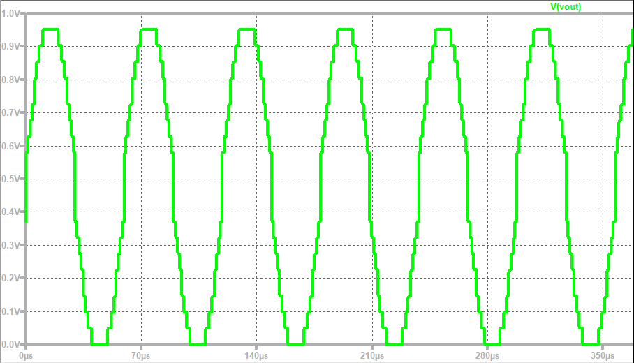
Sine test simulation with LTSPICE.The same error as in the ramp test can be seen here.In the middle of the wave is a bigger step than it should be. |
|
INL and DNL with rampRamp test simulation with INL and DNL calculated by the provided Javascript program.The INL and DNL errors are due to the change of the resistance. This simulates the real behaviour of a DAC, because in reality the resistances are not exactly the nominal value. |

|
Sine test simulationSine test simulation with extracted data and histogram calculated by the providedJavascript program. |

|