Elektronik 320 Datenwandler KennwerteProf. Dr. Jörg Vollrath19 Datenwandler |

|
Video der 20. Vorlesung 15.12.2021
|
Länge: 1:02:43 |
0:0:0 DAC Eigenschaften 0:1:18 Kennlinie und Tabelle DAC 0:3:3 Operationsverstärker für Anpassung Ausgangsbereich 0:4:50 Offset 0:6:54 Gain Error 0:8:45 LSB real 0:10:0 DAC Sinussignal 0:13:10 Formel zur Erzeugung eines Sinussignals 0:16:29 Sinus Lookup Table 0:18:22 Wie sehen Signale bei verschiedene Frequenzen aus 0:19:32 Aliasing, Perioden = 31 und = 1 sehen bei 32 Abtastpunkten gleich aus 0:21:50 Beispiel: LSB, Vout=2 V mit Vref=3.3V N=10 Bit 0:23:10 LSBabs 0:27:30 Genauigkeit LSB 0:30:20 Codeberechnung 0:38:30 Kalibrierung DAC 0:41:30 Konvertierung in Dualzahl 0:44:30 ADC Kenngrößen 0:45:58 ADC Kennlinie und Tabelle 0:50:0 Beispiel LSB 0:50:50 LSBabs und LSBrel 0:53:25 Kalibrierung ADC 0:55:52 Kennlinie, Offset, Gain Error 0:58:1 Beispiel Multimeter 0:59:35 Maximaler und minimaler Code 1:3:20 LTSPICE Model Skalierbarer 4-Bit DAC 1:6:5 LTSPICE Model Skalierbarer 4-Bit ADC 1:6:35 LTSPICE Test |
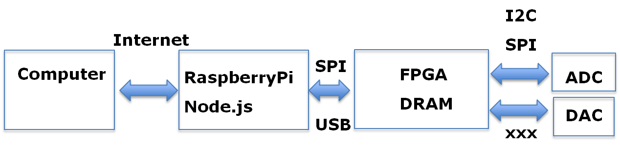
Characterization System
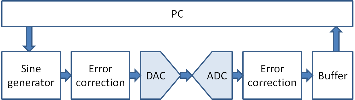

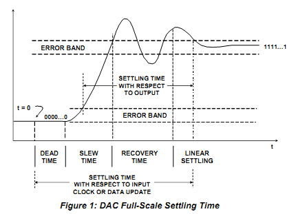
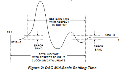
DAC Settling Time
|
|
Quantization Error
|
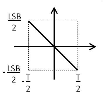
Quantization error is the difference between the quantized signal and the original signal. The quantization error stays between \( \pm \frac{1}{2} LSB \) for the input range. 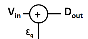 |
|
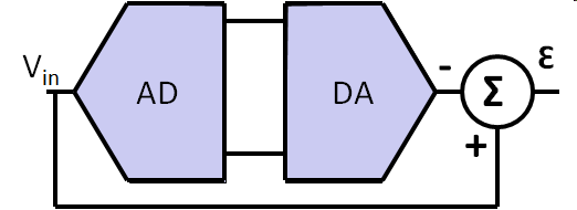
Quantization error can be modeled adding an extra signal εq to the original signal.
ADC dynamic range
|
First approximation: Vsp: signal peak full scale voltage Vqp: peak quantization noise voltage \( SNR \approx 20 \cdot log\frac{V_{sp}}{V_{qp}} \) \( SNR \approx 20 \cdot log\frac{LSB \cdot 2^{N}}{LSB} dB \) \( SNR = 20 \cdot N \cdot log(2) \) \( SNR = 6.02 \cdot N dB\) |
|
ADC dynamic range
|
Second approximation: \( SQNR = 6.02 \cdot N dB + 1.76 dB \) Using integral over quantization error function. \( \overline{\epsilon_{q}^2} = \frac{1}{T} \int_{- \frac{T}{2}}^{+\frac{T}{2}} ( k \cdot t )^2 dt \) |
|
Root mean square value for quantization error is calculated with the integral
over one period T, when the quantization error goes from \( +\frac{T}{2} \)
to \( -\frac{T}{2} \):
\( \overline{\epsilon_{q}^2} = \frac{1}{T} \int_{- \frac{T}{2}}^{+\frac{T}{2}} ( k \cdot t )^2 dt \)
with \( k = - \frac{LSB}{T} \) giving \( T = - \frac{LSB}{k} \):
\( \overline{\epsilon_{q}^2} = - \frac{k}{LSB} \int_{+ \frac{LSB }{2 \cdot k}}^{- \frac{LSB}{2 \cdot k}} ( k \cdot t )^2 dt = - \frac{k^3}{LSB} \left( - \frac{LSB^{3}}{8 \cdot 3 \cdot k^3} - \frac{LSB^{3}}{8 \cdot 3 \cdot k^3} \right) = \frac{LSB^2}{12}\)
\( \epsilon_{q} = \frac{LSB}{\sqrt{12}} \)
\( SQNR = 20 \cdot log \frac{\frac{1}{\sqrt{2}} \frac{LSB \cdot 2^{N}}{2}}{\frac{LSB}{\sqrt{12}}} dB = 20 \cdot log \frac{\sqrt{12}\cdot 2^{N}}{2 \cdot \sqrt{2}} dB \)
\( SQNR = 20 \cdot log \left( 2^{N} \sqrt{\frac{3}{2}} \right) dB = N \cdot 20 \cdot log (2) dB + 20 \cdot log \left( \sqrt{\frac{3}{2}} \right) dB \)
\( SQNR = 6.02 \cdot N dB + 1.76 dB \)
Data converter classification
|
|
FFT simulator
|
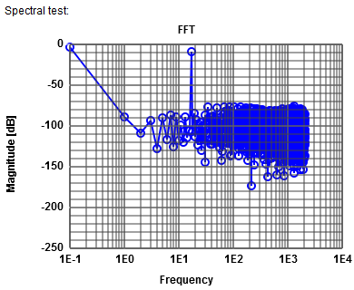
The JavaScript simulator can be used: ADCharacteristic 8-bit ADC, 0.5 V Amplitude, 0.5 V offset, 17 periods, 4096 points FFT. Lowest frequency shows in this simulation DC magnitude. Signal magnitude is -9 dB for frequency 17: 500 mV amplitude gives \( 20 \cdot log \left( \frac{0.5}{\sqrt{2}} \right) = -9 dB \) Total noise is -58 dB which is -9 dB - 6.02*8 dB -1.76 dB = -58 dB using 8 bits. Since the noise is distributed over 4096 bins the noise is distributed around: -58 dB - 10 log (2048) dB = -91 dB. Unfortunately there is a lot of noise, so it is difficult to estimate the -91 dB. |
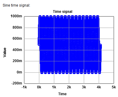  |
Experiments using 8 bits resolution:
16 times the number of ADC levels are used as number of samples for FFT.
28 · 16 = 4096 samples for FFT.
INL is -2.5 and could be centered.
FFT without windowing shows a signal level at fsignal of -9 dB and a harmonic at 2 fsignal with -48 dB.
This gives an ENOB of (-9 dB - (-48 dB) - 1.76 dB) / 6.02 dB = 6 bits.
As expected the random INL will vary with every simulation run. Maximum absolute INL is around 3.
FFT without windowing shows a signal level at fsignal of -9 dB and a total noise level of -34 dB.
This gives an ENOB of (-9 dB - (-34 dB) - 1.76 dB) / 6.02 dB = 4 bits.
8 bits and 17 periods simulation.
Distortion start 0.49, distortion length 0.0036 and distortion amplitude of 0.004.
INL and DNL is 0.9 LSB. Noise floor is 58.13 dB compared to 58.23 dB.
Distortion start 0.49, distortion length 0.0078 and distortion amplitude of 0.01.
From INL and DNL the value of -2 LSB is critical. Noise floor is 56.88 dB compared to 58.23 dB.
Very precise INL, DNL and FFT measurements are needed to catch missing codes.
ω is ω + δ and ω - δ
16 times the number of ADC levels are used as number of samples for FFT.
28 · 16 = 4096 samples for FFT.
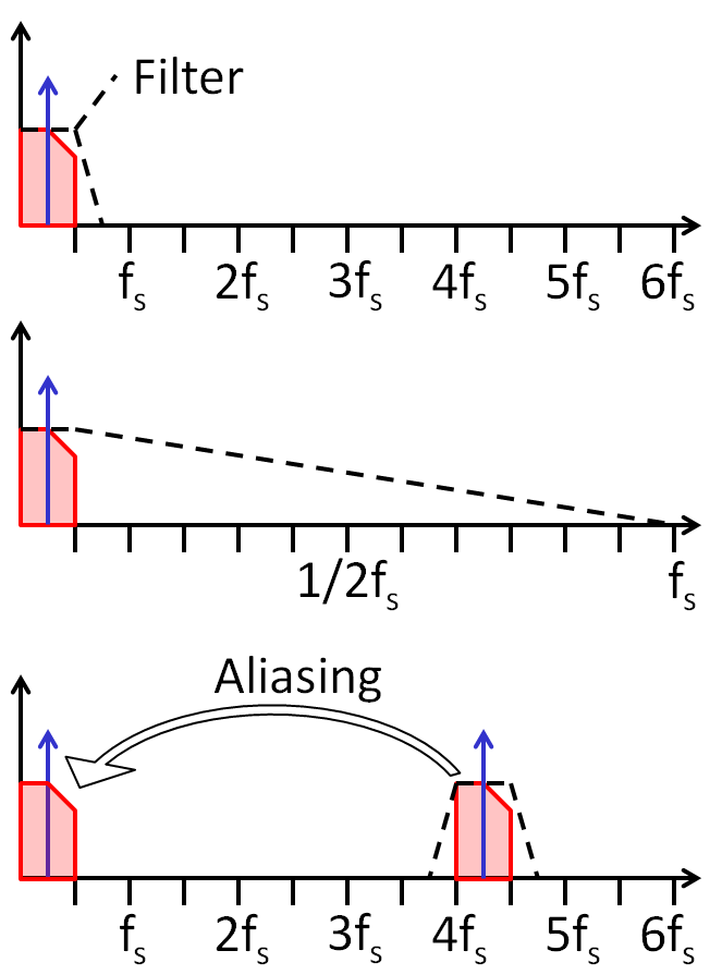
Aliasing
- Number of periods 4096+17 = 4113Bleeding
- Non integer number of periods shows bleeding.Windowing
- Windowing reduces bleeding. The signal peak is distributed over some bins and the magnitude a little reduced.Noise pattern
- Non prime integer number of periods shows noise pattern.DNL, INL and spectral analysis
Errors: Sine amplitude 0.01 is 1 %. It is expected to loose more than 1 bit.INL is -2.5 and could be centered.
FFT without windowing shows a signal level at fsignal of -9 dB and a harmonic at 2 fsignal with -48 dB.
This gives an ENOB of (-9 dB - (-48 dB) - 1.76 dB) / 6.02 dB = 6 bits.
White noise
A noise of 0.01 shows no clear steps in the transfer characteristic any more.As expected the random INL will vary with every simulation run. Maximum absolute INL is around 3.
FFT without windowing shows a signal level at fsignal of -9 dB and a total noise level of -34 dB.
This gives an ENOB of (-9 dB - (-34 dB) - 1.76 dB) / 6.02 dB = 4 bits.
Single distortion in INL, DNL
What happens with the error, if there is one bad conversion.8 bits and 17 periods simulation.
Distortion start 0.49, distortion length 0.0036 and distortion amplitude of 0.004.
INL and DNL is 0.9 LSB. Noise floor is 58.13 dB compared to 58.23 dB.
Distortion start 0.49, distortion length 0.0078 and distortion amplitude of 0.01.
From INL and DNL the value of -2 LSB is critical. Noise floor is 56.88 dB compared to 58.23 dB.
Very precise INL, DNL and FFT measurements are needed to catch missing codes.
Amplitude modulation
Windowing is like amplitude modulation spreading the power:ω is ω + δ and ω - δ