Quantization Error
|
Quantization error is the difference between the quantized signal and the original signal. The quantization error stays between \( \pm \frac{1}{2} LSB \) for the input range. 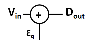 |
 |
Quantization error can be modeled adding an extra signal εq to the original signal.
ADC dynamic range
|
First approximation: Vsp: signal peak full scale voltage Vqp: peak quantization noise voltage \( SNR \approx 20 \cdot log\frac{V_{sp}}{V_{qp}} \approx 20 \cdot log\frac{LSB \cdot 2^{N}}{LSB} dB \) \( SNR = 20 \cdot N \cdot log(2) = 6.02 \cdot N dB\) |
|
ADC dynamic range
|
Second approximation: \( SQNR = 6.02 \cdot N dB + 1.76 dB \) Using integral over quantization error function. \( \overline{\epsilon_{q}^2} = \frac{1}{T} \int_{- \frac{T}{2}}^{+\frac{T}{2}} ( k \cdot t )^2 dt \) |
|
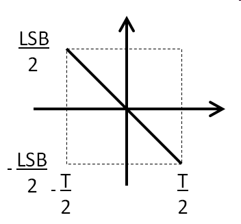
Root mean square value for quantization error is calculated with the integral
over one period T, when the quantization error goes from \( +\frac{T}{2} \)
to \( -\frac{T}{2} \):
\( \overline{\epsilon_{q}^2} = \frac{1}{T} \int_{- \frac{T}{2}}^{+\frac{T}{2}} ( k \cdot t )^2 dt \)
with \( k = - \frac{LSB}{T} \) giving \( T = - \frac{LSB}{k} \):
\( \overline{\epsilon_{q}^2} = - \frac{k}{LSB} \int_{+ \frac{LSB }{2 \cdot k}}^{- \frac{LSB}{2 \cdot k}} ( k \cdot t )^2 dt = - \frac{k^3}{LSB} \left( - \frac{LSB^{3}}{8 \cdot 3 \cdot k^3} - \frac{LSB^{3}}{8 \cdot 3 \cdot k^3} \right) = \frac{LSB^2}{12}\)
\( \epsilon_{q} = \frac{LSB}{\sqrt{12}} \)
\( SQNR = 20 \cdot log \frac{\frac{1}{\sqrt{2}} \frac{LSB \cdot 2^{N}}{2}}{\frac{LSB}{\sqrt{12}}} dB = 20 \cdot log \frac{\sqrt{12}\cdot 2^{N}}{2 \cdot \sqrt{2}} dB \)
\( SQNR = 20 \cdot log \left( 2^{N} \sqrt{\frac{3}{2}} \right) dB = N \cdot 20 \cdot log (2) dB + 20 \cdot log \left( \sqrt{\frac{3}{2}} \right) dB \)
\( SQNR = 6.02 \cdot N dB + 1.76 dB \)
Frequency Domain: Aliasing
|
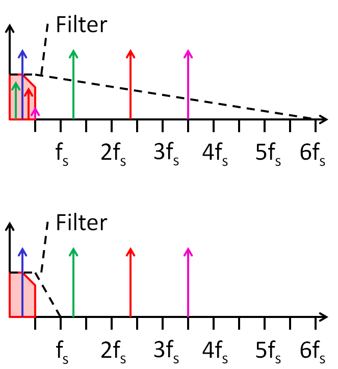
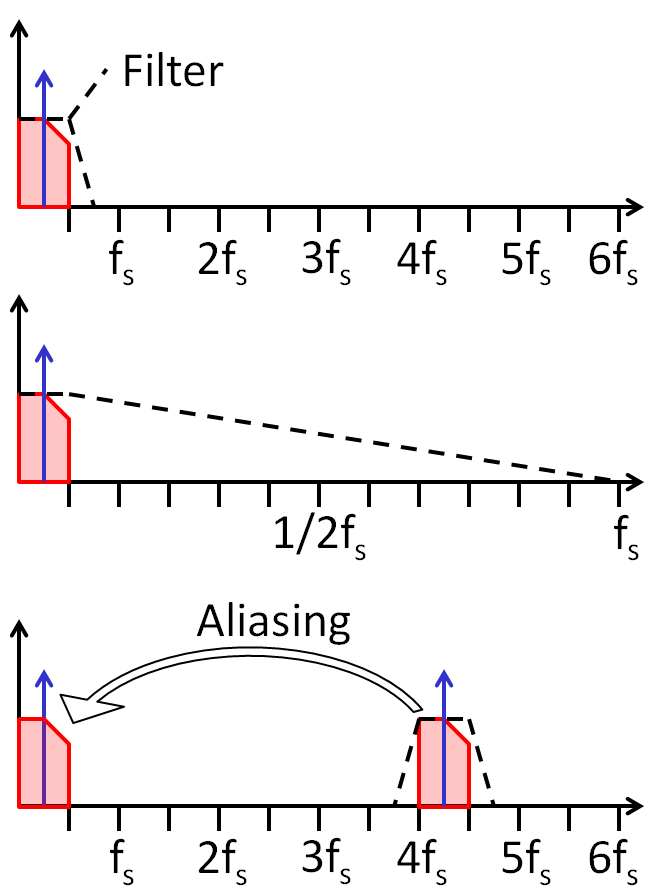
The frequencies fx and nfs ± fx, n integer, are indistinguishable in the discrete time domain Nyquist zones 1st: 0..fs/2; 2nd: fs/2..fs; 3rd: fs..3/2fs; 4th: 3/2 fs..2fs Anti aliasing filter |
|
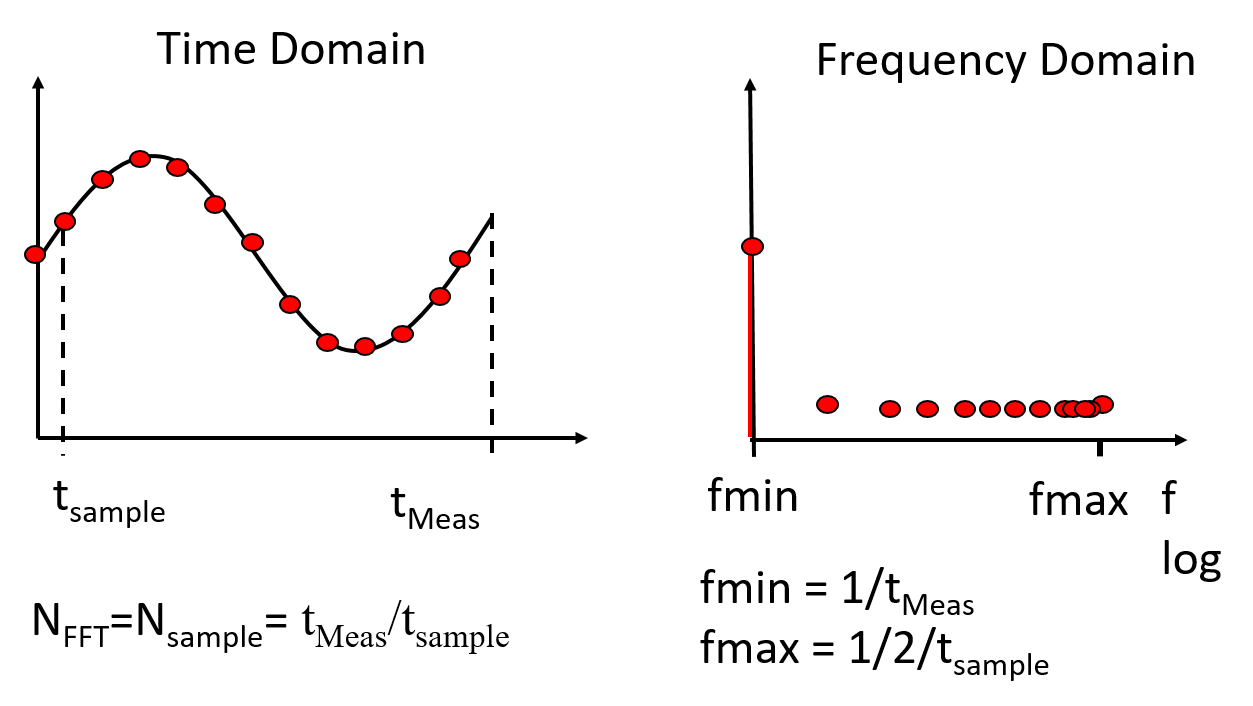
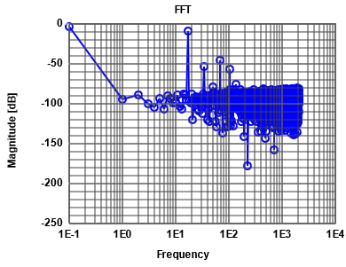
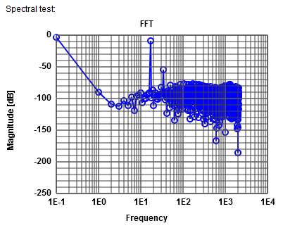
Having a sampling frequency fS gives a frequency spectrum from 0 to fS/2.
Only this range of interested is highlighted in the figures.
The number of sampled points NFFT gives the minimum frequency and the frequency resolution:
fmin = fstep = fS * 2 / NFFT
The figure shows a linear scaling of the frequency x-axis.
Most of the time a logarithmic frequency scaling is used.
Only this range of interested is highlighted in the figures.
The number of sampled points NFFT gives the minimum frequency and the frequency resolution:
fmin = fstep = fS * 2 / NFFT
The figure shows a linear scaling of the frequency x-axis.
Most of the time a logarithmic frequency scaling is used.
Time and frequency domain
 Total noise is distributed to all bins:
\( V_{noise,total} = \sqrt{\sum_1^{\frac{NFFT}{2}} (v_{noise,i})^2} \) \( \Delta a = 10 log \left( \frac{NFFT}{2} \right) dB \)
Data converter classification
|
|
FFT simulator
|
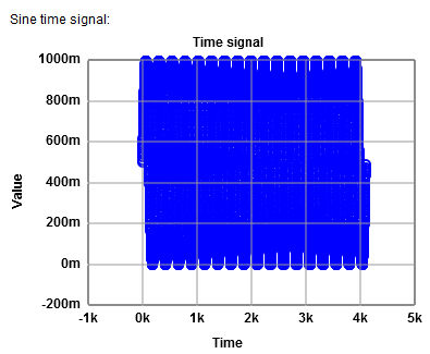
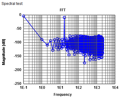
The JavaScript simulator can be used: ADCharacteristic 8-bit ADC, 0.5 V Amplitude, 0.5 V offset, 17 periods, 4096 points FFT. Lowest frequency shows in this simulation DC magnitude. Signal magnitude is -9 dB for frequency 17: 500 mV amplitude gives \( 20 \cdot log \left( \frac{0.5}{\sqrt{2}} \right) = -9 dB \) Total noise is -58 dB which is -9 dB - 6.02*8 dB -1.76 dB = -58 dB using 8 bits. Since the noise is distributed over 4096 bins the noise is distributed around: \( -58 dB - 10 log \left( \frac{NFFT}{2} \right) dB \) = -58 dB - 10 log (2048) dB = -91 dB Unfortunately there is a lot of noise, so it is difficult to estimate the -91 dB. |
  |
Experiments using 8 bits resolution:
16 times the number of ADC levels are used as number of samples for FFT.
28 · 16 = 4096 samples for FFT.
INL is -2.5 and could be centered.
FFT without windowing shows a signal level at fsignal of -9 dB and a harmonic at 2 fsignal with -48 dB.
This gives an ENOB of (-9 dB - (-48 dB) - 1.76 dB) / 6.02 dB = 6 bits.
As expected the random INL will vary with every simulation run. Maximum absolute INL is around 3.
FFT without windowing shows a signal level at fsignal of -9 dB and a total noise level of -34 dB.
This gives an ENOB of (-9 dB - (-34 dB) - 1.76 dB) / 6.02 dB = 4 bits.
8 bits and 17 periods simulation.
Distortion start 0.49, distortion length 0.0036 and distortion amplitude of 0.004.
INL and DNL is 0.9 LSB. Noise floor is 58.13 dB compared to 58.23 dB.
Distortion start 0.49, distortion length 0.0078 and distortion amplitude of 0.01.
From INL and DNL the value of -2 LSB is critical. Noise floor is 56.88 dB compared to 58.23 dB.
Very precise INL, DNL and FFT measurements are needed to catch missing codes.
ω is ω + δ and ω - δ
FFT Playground
16 times the number of ADC levels are used as number of samples for FFT.
28 · 16 = 4096 samples for FFT.
Aliasing
- Number of periods 4096+17 = 4113Bleeding
- Non integer number of periods shows bleeding.Windowing
- Windowing reduces bleeding. The signal peak is distributed over some bins and the magnitude a little reduced.Noise pattern
- Non prime integer number of periods shows noise pattern.DNL, INL and spectral analysis
Errors: Sine amplitude 0.01 is 1 %. It is expected to loose more than 1 bit.INL is -2.5 and could be centered.
FFT without windowing shows a signal level at fsignal of -9 dB and a harmonic at 2 fsignal with -48 dB.
This gives an ENOB of (-9 dB - (-48 dB) - 1.76 dB) / 6.02 dB = 6 bits.
White noise
A noise of 0.01 shows no clear steps in the transfer characteristic any more.As expected the random INL will vary with every simulation run. Maximum absolute INL is around 3.
FFT without windowing shows a signal level at fsignal of -9 dB and a total noise level of -34 dB.
This gives an ENOB of (-9 dB - (-34 dB) - 1.76 dB) / 6.02 dB = 4 bits.
Single distortion in INL, DNL
What happens with the error, if there is one bad conversion.8 bits and 17 periods simulation.
Distortion start 0.49, distortion length 0.0036 and distortion amplitude of 0.004.
INL and DNL is 0.9 LSB. Noise floor is 58.13 dB compared to 58.23 dB.
Distortion start 0.49, distortion length 0.0078 and distortion amplitude of 0.01.
From INL and DNL the value of -2 LSB is critical. Noise floor is 56.88 dB compared to 58.23 dB.
Very precise INL, DNL and FFT measurements are needed to catch missing codes.
Amplitude modulation
Windowing is like amplitude modulation spreading the power:ω is ω + δ and ω - δ
FFT Playground
FFT Table
|
|
The table shows the frequencies sorted by magnitude.
5 harmonics can be seen in thegraph.
5 harmonics can be seen in thegraph.
FFT Application Spectrum
|
|
A simulation is shown:
(8-bit, 17 periods, nonlinearity sine amplitude 0.005, 1 period)
The lowest frequency shows the DC content.
The signal at frequency 17 has -9 dB magnitude.
The first harmonic at frequency 34 has -55.15 dB magnitude.
The average noise level is -82 dB giving a total noise of -59 dB (without Harmonic of -58 dB).
ADC characteristic can be determine:
Since there is only one harmonic SDR and SFDR is the same.
Signal to distortion ratio (SDR): signal to total distortion power (all harmonics).
\( SDR = 10 \cdot \log \left( \frac{Signal \; power}{Total \; distortion \; power}\right) \)
Signal to distortion ratio (SNDR): signal to noise and distortion power.
\( SNDR = 10 \cdot \log \left( \frac{Signal \; power}{Noise \; and \; distortion \; power}\right) \)
Spurious free dynamic range (SFDR): signal to highest harmonic.
\( SFDR = 10 \cdot \log \left( \frac{Signal \; power}{Largest \; harmonic \; power}\right) \)
The objective should be to have all numbers the same getting the expected ENOB.
Harmonics should be eliminated correcting non linearities.
Harmonics can also be eliminated, if the power supply during conversion is not stable.
Non harmonic peaks can come from the power supply or radio interference.
The total noise without harmonics can be increaed due to device parameters: high resistors, low capacitance values, high transistor or operational amplifier input noise.
Diagnosis tries to determine the exact root cause for errors to guide the circuit designer to a better design.
Unfortunately there is little literature available about diagnosis strategies.
(8-bit, 17 periods, nonlinearity sine amplitude 0.005, 1 period)
The lowest frequency shows the DC content.
The signal at frequency 17 has -9 dB magnitude.
The first harmonic at frequency 34 has -55.15 dB magnitude.
The average noise level is -82 dB giving a total noise of -59 dB (without Harmonic of -58 dB).
ADC characteristic can be determine:
| Signal to noise ratio: | SNR = -9.06 dB - (- 59 dB) = 50 dB. Signal magnitude line 1 and total noise magnitude line 2. From there on total noise magnitude remains constant. No more harmonics. |
| Signal to distortion ratio: | SDR = -9.06 dB - (-55.15 dB) = 46.09 dB Signal magnitude line 1 and signal magnitude line 2. |
| Signal to noise and distortion ratio: | SNDR = - 9.06 dB - (- 53.66 dB) = 44.6 dB line 1 |
| Spurious free dynamic range: | SFDR = -9.06 dB - (- 55.15 dB) = 46.09 dB Signal magnitude line 1 and signal magnitude line 2. |
Signal to distortion ratio (SDR): signal to total distortion power (all harmonics).
\( SDR = 10 \cdot \log \left( \frac{Signal \; power}{Total \; distortion \; power}\right) \)
Signal to distortion ratio (SNDR): signal to noise and distortion power.
\( SNDR = 10 \cdot \log \left( \frac{Signal \; power}{Noise \; and \; distortion \; power}\right) \)
Spurious free dynamic range (SFDR): signal to highest harmonic.
\( SFDR = 10 \cdot \log \left( \frac{Signal \; power}{Largest \; harmonic \; power}\right) \)
The objective should be to have all numbers the same getting the expected ENOB.
Harmonics should be eliminated correcting non linearities.
Harmonics can also be eliminated, if the power supply during conversion is not stable.
Non harmonic peaks can come from the power supply or radio interference.
The total noise without harmonics can be increaed due to device parameters: high resistors, low capacitance values, high transistor or operational amplifier input noise.
Diagnosis tries to determine the exact root cause for errors to guide the circuit designer to a better design.
Unfortunately there is little literature available about diagnosis strategies.
Practical Test

LTSPICE simulation data has no fixed time data step size and is non monotonic.
Oscilloscope data can have many samples per output code.
At the moment the FFT tool uses integer data, since ADCs are generating integer data.
| ADC ideal, DAC Test | Ramp | One sample per code |
| ADC ideal, DAC Test | Ramp | Many samples per code |
| ADC ideal, DAC Test | Sine | One or many samples per code |
| ADC Test, DAC ideal | Ramp | One sample per code with missing codes |
| ADC Test, DAC ideal | Ramp | Many samples per code with missing codes |
| ADC Test, DAC ideal | Sine | Many samples per code with missing codes |
Hochschule für angewandte Wissenschaften Kempten, Jörg Vollrath, Bahnhofstraße 61 · 87435 Kempten
Tel. 0831/25 23-0 · Fax 0831/25 23-104 · E-Mail: joerg.vollrath(at)fh-kempten.de
Impressum